empirical distributions continuous distribution

The exponential distribution

In the real world, exponential distributions come up when we look at a series of events and measure the times between events, which are called interarrival times. If the events are equally likely to occur at any time, the distribution of interarrival times tends to look like an exponential distribution.

CDF(x) = 1 − exp(e, −λx)

complementary CDF (CCDF)

1 − CDF(x) = exp(e, -λx)

The random.expovariate generates random values from an exponential distribution with a given value of λ.

The Pareto distribution

CDF(x) = 1 - exp(x/xm, -α)

The Pareto distribution is named after the economist Vilfredo Pareto, who used it to describe the distribution of wealth (see http://wikipedia.org/wiki/Pareto_distribution). Since then, it has been used to describe phenomena in the natural and social sciences including sizes of cities and towns, sand particles and meteorites, forest fires and earthquakes.

Zipf’s law is an observation about how often different words are used. The most common words have very high frequencies, but there are many unusual words, like “hapaxlegomenon,” that appear only a few times. Zipf’s law predicts that in a body of text, called a “corpus,” the distribution of word frequencies is roughly Pareto.

The random.paretovariate, which generates random values from a Pareto distribution.

Pareto distributions are often the result of generative processes with positive feedback (so-called preferential attachment processes).

The Weibull distribution

CDF(x) = 1 - exp(e, -exp(x/λ, k))

Use random.weibullvariate to generate a sample from a Weibull distribution.

The Weibull distribution is a generalization of the exponential distribution that comes up in failure analysis.

The normal distribution

error function

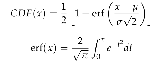
The sigmoid shape of this curve is a recognizable characteristic of a normal distribution. The Bell Curve for pdf, and the sigmoid curve for cdf.

six-sigma

A “six-sigma” event is a value that exceeds the mean by 6 standard deviations.

Normal probability plot

A plot of the sorted values in a sample versus the expected value for each if their distribution is normal.

rankit: The expected value of an element in a sorted list of values from a normal distribution.

The lognormal distribution

CDF-lognormal(x) = CDF-normal(logx)

open data

http://wikipedia.org/

http://mathworld.wolfram.com/

The National Center for Chronic Disease Prevention and Health Promotion conducts an annual survey as part of the Behavioral Risk Factor Surveillance System (BRFSS).

The U.S. Census Bureau publishes data on the population of every incorporated city and town in the United States.

The Internal Revenue Service of the United States (IRS) provides data about income taxes at http://irs.gov/taxstats.

Why model?

Continuous models are also a form of data compression. When a model fits a dataset well, a small set of parameters can summarize a large amount of data.

Generating random numbers

Continuous CDFs are also useful for generating random numbers. If there is an efficient way to compute the inverse CDF, ICDF(p), we can generate random values with the appropriate distribution by choosing from a uni- form distribution from 0 to 1, then choosing x = ICDF(p).

def expovariate(lam):
    p = random.random()
    x = -math.log(1-p) / lam
    return x